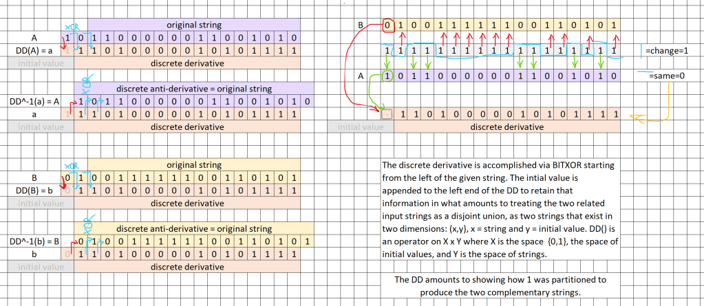
Below are clips of an Excel file that gives a definition of the discrete derivative via an algorithm by which it operates on an infinite binary string….by what it does to an individual string. It also shows how the anti-derivative operates. The discrete derivative is the operator that yields Gray’s code used in porting analog to digital.

An alternate definition is via binary tree. We start with the Binary tree (its vertices are labeled/coded via counting from left to right across a row)…

- The Discrete Derivative (DD) tree is the realization of the algorithm at the top…a set of labels of a binary tree derived from those of the “standard” Binary tree. Note the different vertex labels vs the Binary tree…they follow the new branching pattern from the second row on down (observe the arrows). It has the same form as the Binary tree but the path labels are transformed and therefore so are the codes we get as output from the tree. The DD tree serves as the definition of the discrete derivative when given its simple construction rule below.

- The anti-DD tree is the two together…the vector space some call R as it is…note the different code labels assigned to vertices from the third row on down as compared to both the Binary tree and the DD tree. Note also the difference indicated by the arrows in the third and fourth rows in all three trees.

There are only two “tails” or equivalence classes in the dyadic monoid…they are simply the two infinitesimals corresponding to 0 and 1. The dyadic monoid related to the Stern-Brocot tree links the two fundamental operators (built from the 2×2 matrices a=[[00][10]] and b=[[01][00]]) to the continued fraction form of the real numbers. The intrinsic code in that tree is not a base-two expansion of a dyadic fraction. Rather it is given by simply counting in binary. It encodes the indices of the continued fractions for both finite and infinite continued fractions.
The order we see in the DD tree is the result of either an “external” or “internal” change of a single “bit” between the codes that correspond to indices of continued fractions on adjacent paths. “External” refers to moving 1 up or down from one index to another in a string: adding 1 to one of an adjacent pair of indices while subtracting 1 from the other. A single bit change encodes that. “Internal” refers to partitioning an index by inserting another index of magnitude 1 and thus splitting an index into two parts: one before and one after the new index 1. Again, a single bit change encodes that. Either one results in a single bit change in the coding of the continued fractions between adjacent elements in the ordering. As with a Gray’s coded collection of finite strings, so with the collection of infinite strings represented by paths in the DD tree. The paths are countable: neighbors differ by exactly one bit change.
The only reason we see “uncountable” in Cantor’s diagonal is because we are only looking at the Binary tree. That view ignores the absolutely fundamental role complementation plays in the whole structure. When viewed with your DD/anti-DD glasses on you’ll see that Cantor’s “table” is only the parallel part of a series-parallel partial order.
The very basis of “binary” is complementation: given 0 -> get 1. It cannot be “ignored”. It is the very basis of the logic by which the “proof” is constructed…proof by contradiction. To ignore it is to deny the very basis of proof. These trees are a construction.
The Binary tree is built by complementing 0 to get 1 and then extending that structure repeatedly. All rows are just repeats of the form 0 ->1 all across the row. “Stepping back” we see a self-similar structure. Internally it’s very simple…just a repeat across all rows of 0 ->1.
The DD tree is built by complementing the 0 -> 1 structure of the Binary tree: 0 -> 1, then 1 -> 0 and extending that new 0 ->1_1 ->0 structure repeatedly across all rows. It is the tree version of taking the usual order 00,01,10,11 arrayed as the four corners of a “twisted” unit square (a figure 8) in the first quadrant (00 in the lower left, up to 01, down and to the right to 10, up to 11 and back to 00) and “untwisting” the right side: exchanging places of 10 and 11 to get a new order: 00,01,11,10 and back to 00….going around the square instead of tracing out a figure 8. Equivalently, we can describe the change from 10 ->11 to 11->10 as creating the order noted above: there is exactly one bit change between neighbors as you go round the cycle.
The labels on vertices in each row of the DD tree define a cycle where there is exactly one bit change between neighbors twice as long as that in the prior row. It looks self-similar from the “outside” and is internally rather simple…just a repeat across all rows of 0 ->1_1 ->0. The construction of the DD tree serves as the definition of the discrete derivative. That construction is straight forward as described above. The DD of a string is given by following the steps of a path from the Binary tree (where 101100… = RLRRLL… ) and recording the corresponding labels as shown instead by the DD tree. The result across the whole infinite tree is an automorphism of the collection of paths in the Binary tree.
The anti-DD tree is special. It is fundamentally different from the first two. It is not just an extension across all rows of the same module. It is recursive from row to row. It is internally self-similar and has a complex structure when viewed from “outside”. The order of the arrows as depicted in the tree diagram above seems to change from row to row. Its construction starts by complementing the basic module of the DD tree: 0 ->1_1 ->0 || 1 ->0_0 ->1 but rather than just copying that across every row we repeatedly apply that complementation in subsequent rows by copying a prior row into the next row’s left half and putting its complement in the right half…over and over down the rows….it is not a static form like the other two. We define a second automorphism of the Binary tree by following paths defined in the Binary tree (LLLRRLRLRR…) and recording the new labels assigned in the anti-DD tree.
With the transformations of the Binary tree as defined by the stated constructions of the DD and anti-DD trees we get a chain of relationship between three trees of strings…a three element group of automorphisms of the Binary tree.
The fine structure of the transformation from Binary to DD to anti-DD is shown in the diagram below. We see there a cyclic group with three elements that produces unordered triples (a,b,c) of strings. They are the parallel in “series-parallel”. Those triples are linked via the ordered triples (A,B,C)… the series part of the order. The DD of a “seed” is the “seed’ for another DD string. The anti-DD of a “seed” is the “seed” of the DD that results in the “seed” as well as the DD of another “seed” before it…and so on. Sounds confusing…look at the graphic below.

The whole structure is built on complementation but with a fundamental role for self-similarity. All three trees exhibit a kind of self-similarity as viewed from “outside”…in their entirety. Only the anti-DD tree is internally self-similar as stated in the description of its construction.
Complementation and self-similarity are the two kinds of “reflection”:
- In the mirror my reflection has his phone in his left hand while I have mine in my right.
- When my identical twin with his phone in his right hand faces me across the boundary between us I see he has his phone in his right hand just like me.
They are properly referred to as:
- Affine…the curl of the field…00,01,10,11…around the square…the reflection is parallels…there is a discontinuity at the return to 00 from 11…the point at infinity is missing…2 bits change
- Projective…the divergence of the field…00,01,11,10…along the diagonals…00-01-11-10 and back to 00 involves always exactly one bit change: continuity…never more than one bit changes….the “reflection” is really a crossing over to the other “side”.
From the Wiki page on Affine space: “Bob sees only the affine structure. Alice sees both the affine and projective structure.”
If all you see is the affine structure R looks “uncountable”. When viewed as both affine and projective one sees that is not the case. The structure is far simpler in ways and far deeper in others. What one sees is a projective space that produces an affine space where we find parallels that don’t meet and a missing point at infinity. The consequences extend into an arithmetic that is built on an affine view.
When we “import” the “0” into the multiplicative group built on the two generators (the 2×2 matrices L=[[10],[11]] R=[[11],[01]]) that generate the Stern-Brocot tree… (all the vectors with integer components -> all the directions with rational tangents)…to get our “field” in affine space where there is no element for division by 0 (as in projective space…the point at infinity)…we import incompleteness…division becomes a partial function.
All the King’s horses and all the King’s men have not been able to put Humpty back together again.
Put the three trees into perspective and one understands why. The two equivalence classes we get in the coding (the Stern-Brocot tree) are nothing more than infinite strings with the same “tail”, either infinitesimal 0 or 1 (a or b), with a range of prefixes: Q. Those tails are the indeterminate “ends” attached to the finite strings that make up Q….they are what turns those finite strings into “infinite” strings…they are the one step beyond Q, beyond finite….and there is only one.
The 00000…string (the infinite string of 0’s) is the fixed point of the DD and anti-DD trees. It runs down the left side of all the trees and is never “relocated”.
